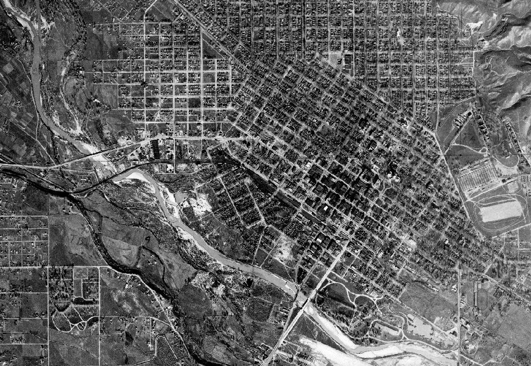

Since we can see that there was a substantial amount of the development outside of the city limits boundaries we need to zoom out and consider the local government body that s responsible for these areas. In this case, that is the county government.
The previous research on land use change that have looked at county governments have found that the county government land use regulations have effectively controlled sprawling land use development.
However, some researchers have found that not all county government are the same. This issue makes it difficult to generalize the results from one county to another. But they exhibit two types of patterns in terms of scope of power. The first pattern consists of strong county governments that share land use change regulation responsibilities with a single large municipal government. The second pattern is a county government that is responsible for the unincorporated areas and then shares responsibilities in certain areas with several different smaller municipalities.
d. The previous research has focused on the first pattern of county government. That is, the strong county government that shares regulatory responsibilities with a large municipality. This focus has been at the expense of understanding the second pattern.
This leads me to my contribution which is that I look at the county government that fits the second pattern and see if it is an effective driver of land use change. Additionally, I use the regression discontinuity design which provides better support for causal claims than basic regression analysis. I will review the RDD when I discuss my data and methods.
The area that I look at in my research is the Treasure Valley. And the treasure valley offer an excellent opportunity to study land use change regulation because the two counties, Ada and Canyon, are set up like natural experiment. For instance, since both counties are in the Treasure Valley, they can be expected to share many environmental and geographic qualities. The way in which the two counties differ is in their planning activities. For the period that I am looking, 2001 to 2011, Ada County has been active in developing plans for future development whereas canyon county has been much less active. Therefore, since the two counties share similar environmental and geographic qualities, we potentially can attribute the difference in land use change between the two counties to planning activities.

↘

↗

↖

←

↙

↓

↘

→

↗
To test the effectiveness of the Ada County government in driving land use change, I follow the recent land use change literature and use the optimal timing of development model. This theory suggests that land owners or developers will change the land use of their parcel if they find that it maximizes their utility. Additionally, land owners will change the land use of their parcels when they find that the cost of waiting outweighs the benefits.
Using this theory in the context of Ada County, I have two hypotheses that I test. For both hypothesis, I expect that Ada County will have a discernible effect on land use change that fits the Blueprint policies. But for each hypothesis, I assume a different level of enforcement intensity. For the first hypothesis, I assume that Ada County will be a strong enforcer of land use change regulation. What I mean by this is that I assume that Ada County will try to restrict change in land use from undeveloped to developed as much as possible. Specifically, I first hypothesize that if a parcel is in Ada County, then the parcel is less likely to change land use from an undeveloped land use to a developed land use than a parcel in Canyon County.
For the second hypothesis, I assume that Ada County will be less strict in enforcing land use change but will still encourage it in impact areas. So, secondly, I hypothesize that if a parcel is in Ada County, then it is more likely to change land use from undeveloped to developed if it is located within a designated city impact area.
Therefore, the null hypothesis in this case that the Ada County government will not an affect land use change Ada County.
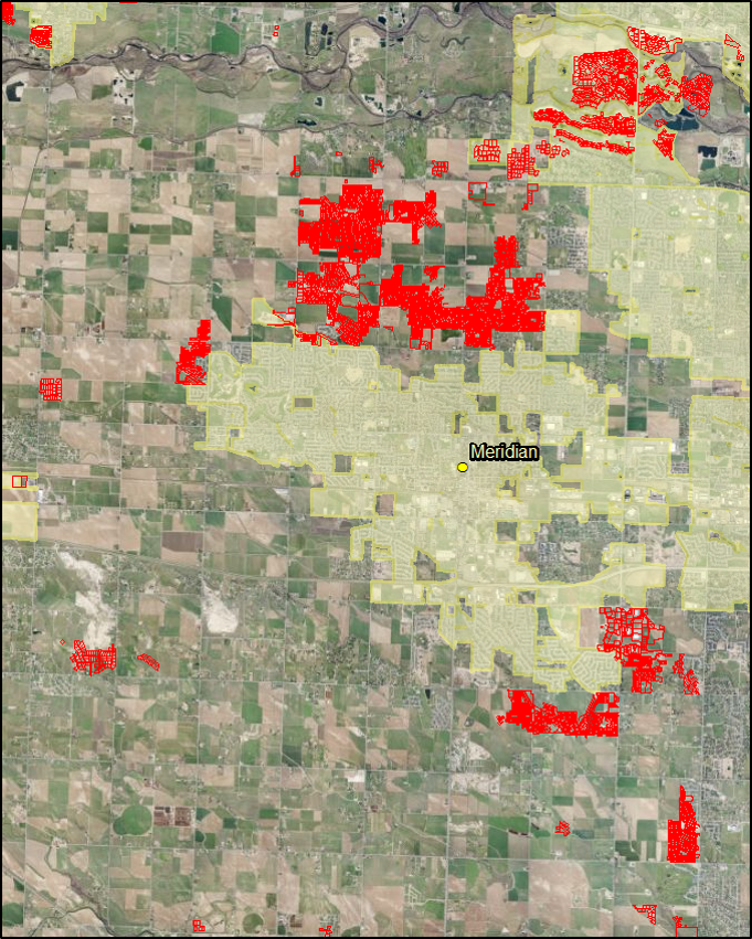
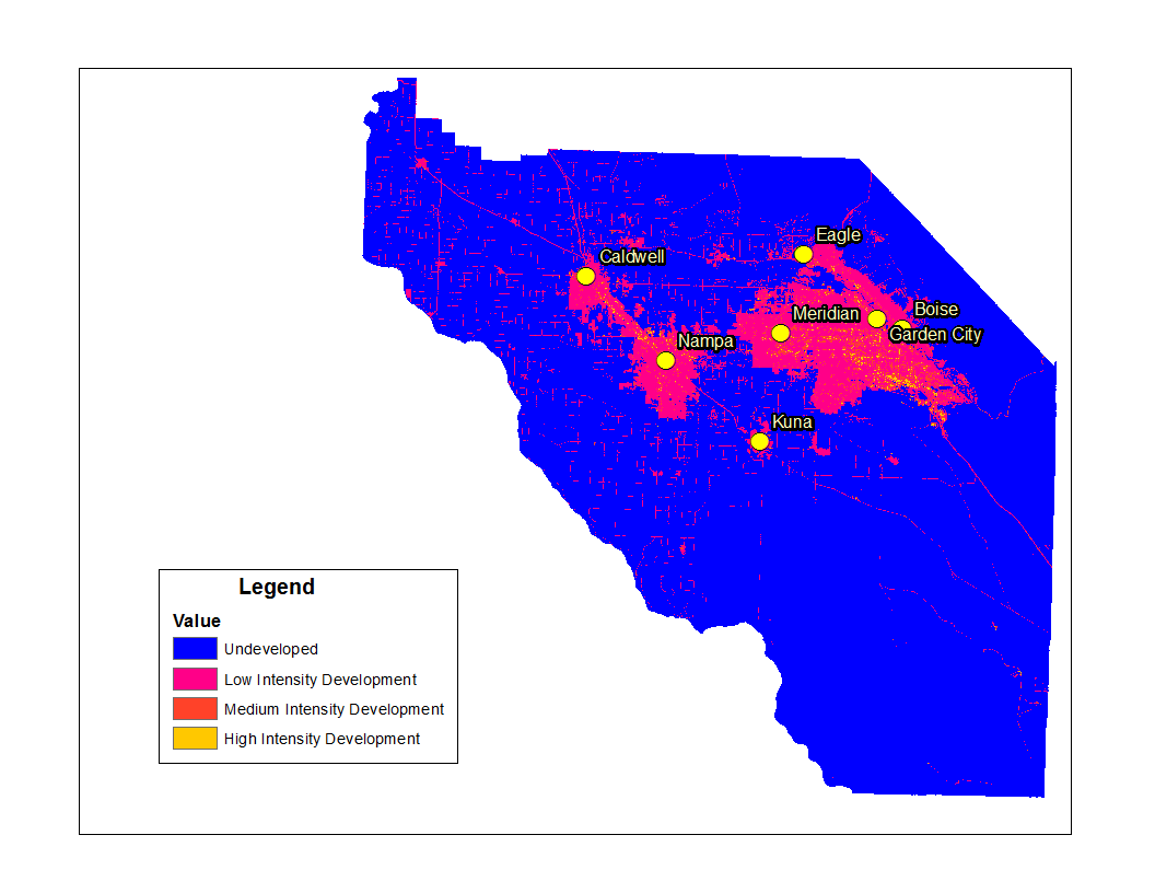
To test my hypotheses, I use a dataset of nearly 89 thousand parcels that are undeveloped as of 2001. This dataset contains information on each parcel that includes whether the parcel changed land use, its size, its distance to geographic features and the population density of the area it is in.
Here is an image of all the parcels included in the dataset. The ones in blue are those that changed land use from 2001 – 2011.
There are six dependent variables that I use to estimate the effect that Ada County has on land use change. The dependent variables were created using NLCD land cover layers for the three years available. The dependent variables are first separated by type. Three of the dependent variables are binary and they capture whether a parcel changes land use from undeveloped to developed. The other three are categorical and capture land use change from undeveloped to a specific developed land use. For instance, a parcel receives a value of 1 if it changed from undeveloped to low intensity development, a 2 if it changed to medium intensity development and a 3 if changed to a high intensity development. A parcel receives a zero if it did not change land use and this is the case for the both the binary and categorical dependent variables. The reason that I use two different discreet dependent variables is because I use two different datasets. The one dataset is based on the RDD which is a smaller subset of the whole dataset. In this dataset the number of occurrence of outcome 2 and 3 are so few that I decided to combine all kinds of development and look at development generally for the parcels included in the RDD dataset. For the whole dataset, I use the categorical dependent variables.
For each type of dependent variable, there is one that captures a different period. For each type, there is one that captures the period from 2001 to 2011. I use this dependent variable to capture the overall trend of land use change. The second one captures land use change from 2001 – 2006. I use this dependent variable to capture the baseline trends. That is, I look at the associations between the land use change and the drivers of land use change before the Blueprint was implemented. The last period captures change from 2006 – 2011. This is the period in which policies from the Blueprint were implemented. Additionally, this is the period my hypotheses address.
| Models | DV Version | Dataset | # of Parcels | Outcome 0 | Outcome 1 | Outcome 2 | Outcome 3 | % Change |
|---|---|---|---|---|---|---|---|---|
| Model 1 | Categorical | 01 - 11 | 88893 | 66516 | 20011 | 2337 | 79 | 25% |
| Model 2 | Categorical | 01 - 06 | 88893 | 67419 | 19351 | 2112 | 61 | 24% |
| Model 3 | Categorical | 06 - 11 | 67434 | 66502 | 910 | 19 | 3 | 1% |
| Model 4 | Binary | RDD, 01 - 11 |
7821 | 6369 | 1452 | - | - | 19% |
| Model 5 | Binary | RDD, 01 - 06 |
7821 | 6369 | 1452 | - | - | 18% |
| Model 6 | Binary | RDD, 06 - 11 |
6369 | 6344 | 25 | - | - | .4% |
So each dependent variable is used in a different model. Models one through three use the categorical dependent variables. The first model uses the categorical variable for the period from 01 – 11 and the entire dataset of undeveloped parcels which equal roughly 89 thousand. Moving across we can see the number of occurrences for each outcome with a total 25% percent of the parcels changing land use for the whole period. The next model uses the categorical variable for the period from 01 – 06 and the entire dataset 89 thousand parcel with 24% of the parcels changing land use for this period. The third model uses the categorical variable for the period from 06 – 11 and it uses a dataset that includes parcels that are undeveloped as of 2006 which equals roughly 67 thousand parcels with one percent changing land use. The last three models use the binary dependent variable. Model 4 uses the binary dependent variable for the period from 01 – 11 and uses the dataset based the RDD which I will get into here in a sec. This dataset includes roughly 78 hundred parcels with 19% percent changing land use. Model 5 uses binary dependent variables for 01 – 06. It uses the same number of parcels with 18 percent changing land use for this period. Model 6 uses the binary dependent variable for the period from 06 – 11 and uses parcels from the RDD dataset that are undeveloped as of 2006 with roughly half percent changing land use.
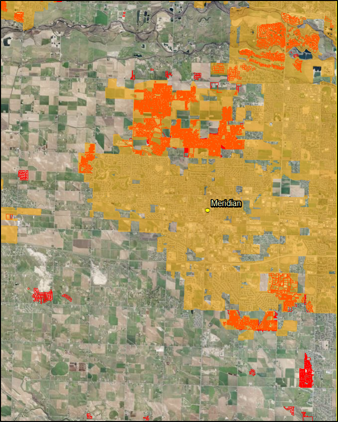
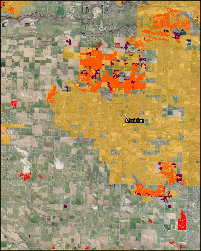
Here is a land use map for the Treasure Valley for the year 2011.
Next are the independent variables and the two primary variables of interest are the county and impact area variables. The county variable is coded to capture the county location of the parcel with a parcel receiving the value of one if it is in Ada County.
The impact area variable is coded to capture whether a parcel is in an impact area with 1 if it is. Since impact areas are of interest because of the Blueprint, the impact area variable is included those models that use the dependent variables for 2006 – 2011.
The hypothesized outcomes for these variables are as follows. For the first hypothesis, which assumes that Ada County is a strong enforcer of land use regulation, the expected outcome is that the coefficient for the county variable will be negative. This means that Ada County will discourage land use change from undeveloped to developed to such an extent that a parcel located in Ada County is less likely to change land use compared to Canyon County.
For the second hypothesis, which assumes that Ada County would be a weak enforcer of land use regulation, the expected outcomes are first that the coefficients for the county and impact area variables will be positive and the impact area variable will have a larger coefficient. This means that if a parcel is more likely to develop in Ada County, it is more likely to change land use if it is in an impact area.
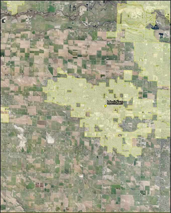
Here is an image of the counties and the impact area.
The other independent variables that I include in each model are parcel size, distance to nearest city, distance to water feature and population density.
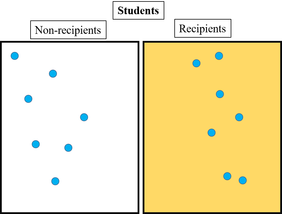
Before I get to my results I am going quickly review the RDD. The RDD is a quasi-experimental design that approximates the experimental design. This means that a subset of a larger sample is taken that includes subjects that are nearly matching. In an experimental design, the subjects are separated into either a control group or a treatment group. Those in the treatment group receive the treatment. Then any difference that exhibited between the two groups is attributed to the treatment. In social science, Thistlethwaite and Campbell introduced the RDD to approximate the experimental design. In their research, they took a sample of students who competed for a national scholarship. They then took a subset of that sample that included students that were nearly matching in several background variables. This subset included both nearly losers and nearly winners of the competition. The students who lost acted as the control group. Those that won were treated like the treatment group because in addition to winning the scholarship the students received a certificate of merit and public attention for winning. In their research, T and C hypothesized that the students who won the scholarship would be more inclined to pursue intellectual careers like those in academia because they receive the award and attention.
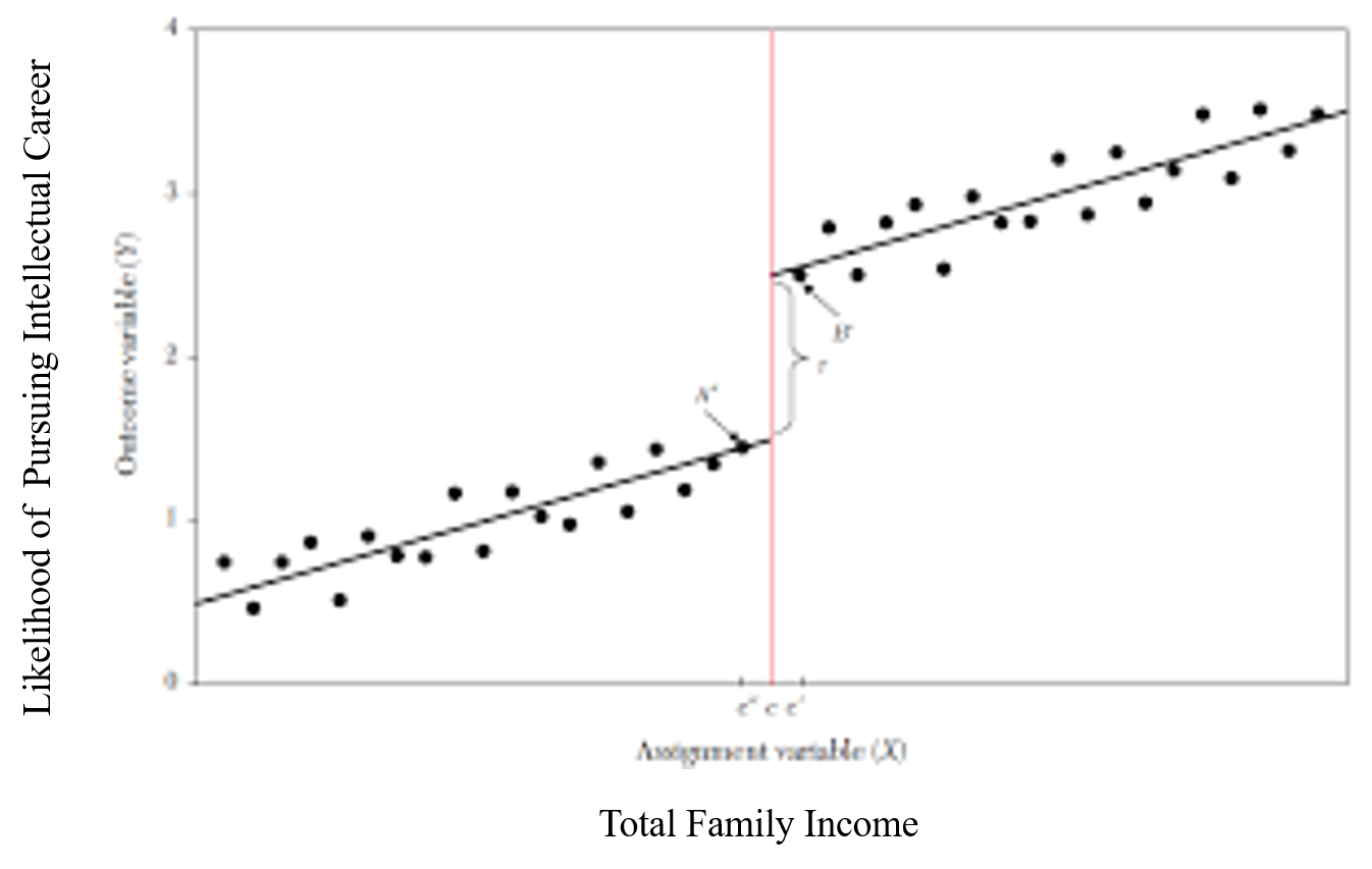
Here is a hypothetical graph of what T and C hypothesized. If we assume that on the x axis there is a background variable such as total family income and on the y axis is some metric for likelihood for pursuing an intellectual career, then we can see that as family income increase so does the likelihood of an academic career. But here in the center is a jump in the trend and this jump is linked to the student receiving the award and attention. To capture this effect, we operationalize the treatment by including a dummy variable that captures whether an observation received the treatment. The coefficient is then a measure of the magnitude of the effect that the treatment has on the outcome of the dependent variable. In this case, the dummy variable would be whether a student received the award and the attention.
The RDD provides better support for causal claims because it limits the amount of the variation in the dependent variable that is explained by unobservables.
The RDD has been utilized a handful of times in the land use change literature. One article used an RDD and found that city zoning ordinaces increased the likelihood that a parcel in Medina County, Ohio will change land use.
The observations in their study were parcels that were located within 25 hundered feet of a city zoning boundary.
The treatment in their study were the zoning ordinances.
To implement the RDD in my research, I chose to include parcels that are within a 1 mile distance from the Ada County and Canyon County border. I chose this distance because it fell within the range of distances used in the previous research. I also did a sensitivity analysis using distances up to two miles without finding any substantial difference between the results. Distances within than a mile eliminated any variation in the dependent variables.
To apply the quasi – experimental mold to my research. My test subjects are nearly matching observations along the border of Ada county and Canyon county. The control group are the parcels in Canyon County. The treatment group are those in Ada County. And the treatment is the blueprint policies implemented in Ada County
Here are the hypothesized outcomes again for the period from 06 – 11. For the first hypothesis, in which I assumed that Ada County is a strong enforcer of land use regulation, I hypothesize that the county variable will be negative because Ada County will discourage a parcel from changing land use to such extent that a parcel in Ada County will be less likely to change. For the second hypothesis, in which I assume that Ada County would be a weak enforcer, I hypothesize that the county and impact area variables will be positive and the coefficient for the impact area variable will be larger. This means that Ada County will not outright discourage land use change within the county but encourage it within impact area.
| Outcomes(Base: 0) | 1 | 2 | 3 | |||
|---|---|---|---|---|---|---|
| β | sig | β | sig | β | sig | |
| County^ | .81 | *** | 1.44 | *** | 1.53 | *** |
| Impact Area^ | - | - | - | - | - | - |
| Parcel Size | -.46 | *** | -.53 | *** | -0.50 | *** |
| Distance to Nearest City | -5.3E-05 | *** | -7.2E-05 | *** | -7.6E-05 | *** |
| Distance to Water Feature | 7.60E-06 | *** | 9.36E-06 | *** | -2.94E-06 | *** |
| Pop. Density | 0.001 | *** | 0.001 | *** | 0.001 | ** |
| Constant | -0.91 | *** | -3.06 | *** | -6.15 | ** |
| Pseudo R2 | 0.28 | |||||
| N | 88893 | |||||
| ***=Significant at 1% | **=Significant at 5% | *=Significant at 10% | ^=Dummy Variable | |||
The results for Model 1 which used the categorical dependent variable for 01 – 11. For each set of results, I have highlighted the primary variables of interest like I have done here. This first model is meant to capture the trends for the whole period and for the entire treasure valley. The results show that all the coefficients are significant at the 1% level for all the outcomes except for population density and distance to water feature for outcome 3. Population density in this case is significant at the 5% level and distance to water feature is not significant at all. The direction of the coefficient hold across all outcomes. For instance, the county variable is positive which indicates that a parcel in Ada County is more likely to change land use than one in Canyon county. Parcel size and Distance to nearest city are both negative which means that if a parcel is larger and far from the nearest city it is less likely to change land use. Population Density and distance to water feature are positive for those coefficients that are statistically significant. This means that parcels more likely to change land use if they are in areas with higher populations and if they are far from a water feature.
| Outcomes(Base: 0) | 1 | 2 | 3 | |||
|---|---|---|---|---|---|---|
| β | sig | β | sig | β | sig | |
| County^ | .81 | *** | 1.37 | *** | 1.69 | *** |
| Impact Area^ | - | - | - | - | - | - |
| Parcel Size | -.44 | *** | -.53 | *** | -0.37 | *** |
| Distance to Nearest City | -5.2E-05 | *** | -7E-05 | *** | -6.8E-05 | *** |
| Distance to Water Feature | 7.38E-06 | *** | 1.01E-05 | *** | 1.9E-05 | *** |
| Pop. Density | 0.001 | *** | 0.0008 | *** | 0.001 | *** |
| Constant | -1.008 | *** | -3.21 | *** | -6.52 | *** |
| Pseudo R2 | 0.27 | |||||
| N | 88943 | |||||
| ***=Significant at 1% | **=Significant at 5% | *=Significant at 10% | ^=Dummy Variable | |||
Here are the results for Model 2 which uses the categorical dependent variable for the period from 01 – 06. This model is meant to capture trends before Blueprint policies are implemented. The results for this model are largely the same as those for Model 1. One exception is the coefficient for distance to water feature for the third outcome which is significant for this model and is in the opposite direction of the two other outcomes. This means that a parcel that is far from a water feature is less likely to change land use from undeveloped to high intensity development.
| Outcomes(Base: 0) | 1 | 2 | 3 | |||
|---|---|---|---|---|---|---|
| β | sig | β | sig | β | sig | |
| County^ | .70 | *** | -3.76 | -13.29 | ||
| Impact Area^ | -.14 | - | 5.05 | - | -1.57 | - |
| Parcel Size | -.22 | *** | -.04 | - | -0.21 | |
| Distance to Nearest City | -6.5E-05 | *** | -5E-05 | - | -0.00027 | - |
| Distance to Water Feature | 7.39E-06 | *** | 3.33E-05 | ** | -.0001 | ** |
| Pop. Density | 0.001 | *** | 0.0008 | * | 0.001 | - |
| Constant | -3.03 | *** | -8.24 | - | -7.16 | - |
| Pseudo R2 | 0.14 | |||||
| N | 67434 | |||||
| ***=Significant at 1% | **=Significant at 5% | *=Significant at 10% | ^=Dummy Variable | |||
Here are the results for Model 3 which uses the categorical dependent variable for the period from 06 – 11 and is one model in which the hypotheses apply. For the first outcome, the coefficient for the county variable is positive which is contrary to hypothesis one. Additionally, this coefficient is positive while the coefficient for the impact area is negative and insignificant which is contrary to hypothesis 2. The county variable is in the right direction for outcome 2 and 3 for the first hypothesis, however, both are insignificant. The impact area variable is also significant for both outcomes and in the wrong direction for outcome three. The results for the remaining variables are similar to the previous two models. However, distance to nearest city and distance to water feature are the only variables that hold significance for all outcomes.
| Outcomes(Base: 0) | 1 | 2 | 3 | |||
|---|---|---|---|---|---|---|
| β | sig | β | sig | β | sig | |
| County^ | .09 | *** | .08 | *** | .003 | *** |
| Impact Area^ | - | - | - | - | -.0007 | - |
| Parcel Size | -.05 | *** | -.04 | *** | -0.001 | *** |
| Distance to Nearest City | -5.44E-06 | *** | -5.11E-06 | *** | -3.16E-07 | *** |
| Distance to Water Feature | 7.75E-07 | *** | 7.31E-07 | *** | 3.57E-08 | *** |
| Pop. Density | 0.001 | *** | 0.00012 | *** | 1.42E-06 | *** |
| ***=Significant at 1% | **=Significant at 5% | *=Significant at 10% | ^=Dummy Variable | |||
Here are the marginal effects for outcome 1 for Models 1 – 3. I didn’t include the marginal effects for other outcomes because all the results were insignificant. The pattern in this set of results is that the marginal effects for models for 1 and 2 are similar and larger than for model three. For instance, for models 1 and 2, a parcel is 8 percent more likely to change land use if it is in Ada County. This effect drops to .3 percent for model three. This pattern holds for the remaining independent variables except impact area which is insignificant and not included in models 1 and 2.
| Model 4 | Model 5 | Model 6 | ||||
|---|---|---|---|---|---|---|
| β | sig | β | sig | β | sig | |
| County^ | 1.03 | *** | 1.03 | *** | 3.24 | *** |
| Impact Area^ | - | - | - | - | -0.99 | - |
| Parcel Size | -.59 | *** | -.59 | *** | -5.64E-01 | *** |
| Distance to Nearest City | -8.6E-05 | *** | -8.6E-05 | *** | -1.25E-04 | *** |
| Distance to Water Feature | -7.4E-05 | *** | -7.4E-05 | ** | -2.9E-05 | *** |
| Pop. Density | 0.002 | *** | 0.002 | *** | -0.01 | *** |
| Constant | 1.23 | *** | 1.23 | *** | -1.18 | - |
| Pseudo R2 | 0.42 | .41 | .32 | |||
| N | 7821 | 7821 | 6369 | |||
| ***=Significant at 1% | **=Significant at 5% | *=Significant at 10% | ^=Dummy Variable | |||
Here are the results for models that use the RDD dataset. Most of the results are similar to those in the previous models. The county variable is positive and significant and the impact area variable is negative and insignificant which contrary to both hypotheses. The results for the remaining variables are in same direction as the previous models except for distance to water feature which is negative for each model. Additionally, population density is also negative for model 6 which differs from model 3 which looks at the same period.
| Outcomes(Base: 0) | 1 | 2 | 3 | |||
|---|---|---|---|---|---|---|
| β | sig | β | sig | β | sig | |
| County^ | .05 | *** | .05 | *** | .002 | * |
| Impact Area^ | - | - | - | - | -.00034 | - |
| Parcel Size | -.02 | *** | -.02 | *** | -0.002 | * |
| Distance to Nearest City | -4.12E-06 | *** | -4.12E-06 | *** | -5.23E-07 | * |
| Distance to Water Feature | -3.53E-06 | *** | -3.53E-07 | *** | -1.20E-08 | - |
| Pop. Density | 0.0001 | *** | 0.0001 | *** | -6.28E-06 | * |
| ***=Significant at 1% | **=Significant at 5% | *=Significant at 10% | ^=Dummy Variable | |||
The marginal effects share the same pattern to those for the previous models. That is, the models that look at the 01 – 11 and 01 – 06 period have larger effects for each variable compared to the model that looks at the period from 06 – 11. Additionally, the results for model six are significant at lower levels than any other model.
For the period from 2006 – 2011, I first hypothesized that the county variable would be negative. This hypothesis assumed that Ada County would be a strong enforcer of land use regulation and discourage land use change as much as possible. However, the results for the county variable were significant and positive. Second, I hypothesized that if county is positive then the impact area will also be positive and the coefficient would be larger for the impact area. For this hypothesis, I assumed that Ada County be a weak enforcer of land use regulation but would encourage development within impact areas. However, the results show that the county variable was often positive and significant and the impact area variable was negative and insignificant.
The results suggest that Ada County was not effective in driving land use change. Additionally, the results also suggest that county governments that fit the second pattern of scope of power over land use regulation are not effective at controlling and steering land use change. The results for the other independent variables suggest that a parcel that is large and far from the nearest city is unlikely to change land use. Additionally, a parcel is more likely to change land use if it is an area with a high population. Finally, the distance to water feature was ambiguous because for the first models a higher distance to a water feature increased the likelihood that a parcel will change land use expect for high intensity development. However, the opposite was the case for those parcels along the border between the counties.